08 — Pixel Histograms and Minkowski Functionals¶
Purpose: Evaluate one-point statistics and morphological properties of DDPM samples against Agora and Gaussian baselines.
This notebook covers two complementary non-Gaussian diagnostics:
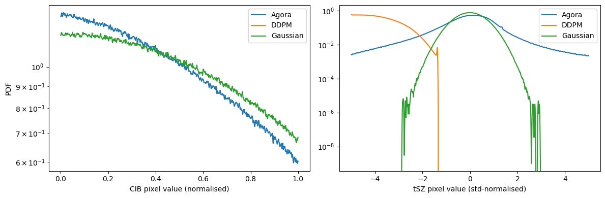
Pixel intensity histograms — normalised histograms of pixel values for 200 CIB and tSZ samples from each source (Agora, DDPM, Gaussian), binned over [0, 100] μK for CIB and [−100, 0] μK for tSZ in 1000 bins and smoothed with a Gaussian kernel (σ = 1). Probes the one-point PDF and highlights the DDPM’s underproduction of extreme-value pixels.
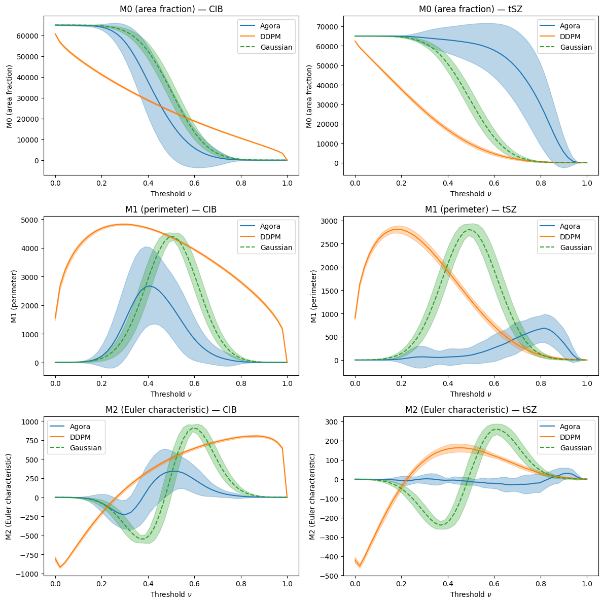
Minkowski functionals — computes M0 (area fraction), M1 (total boundary length), and M2 (Euler characteristic) of excursion sets across 50 intensity thresholds ν ∈ [0, 1] using the Boelens & Tchelepi software package. Applied to min-max normalised maps for CIB and tSZ separately.
Inputs:
Test maps and DDPM samples:
data/low_pass/2mJy/*.npyGaussian baseline:
data/low_pass/2mJy/gaussian_cib_tsz_2mJy_lp.npy
Outputs: pixel histogram plots (Figure 5), Minkowski functional plots (Figure 6).
Key module functions:
foregrounds_diffusion.preprocessing.apply_maxmin_normalizationforegrounds_diffusion.preprocessing.apply_stdnorm
External dependency: minkowski (Boelens & Tchelepi package) for Minkowski functional computation.
Paper reference: §3.2 (statistics definitions), §4.4 (Figure 5), §4.5 (Figure 6).
1 Setup¶
compute_mfs from foregrounds_diffusion.morphology requires the optional quantimpy package (Boelens & Tchelepi 2021). If quantimpy is not available the notebook falls back to a graceful skip of the Minkowski functional section, printing a warning. The pixel histogram section runs without any optional dependency.
Note on quantimpy compatibility: quantimpy 0.2.6 was compiled against NumPy 1.x and raises a
ValueErroron NumPy 2.x. Install NumPy 1.26.4 or rebuild quantimpy from source against the installed NumPy version if compatibility errors are encountered.
[ ]:
import numpy as np
import matplotlib.pyplot as plt
from scipy.ndimage import gaussian_filter1d
from pathlib import Path

from foregrounds_diffusion.preprocessing import apply_maxmin_normalization, apply_stdnorm, renormalize_dm_maps, denormalize_dm_maps
from foregrounds_diffusion.morphology import compute_mfs

PTSRC     = 2
N_MAPS = 200   # number of maps used per source

PROJECT_ROOT = Path("/home/apb86/cmb_foregrounds_diffusion")
PATCHES_DIR = Path(f"data/low_pass/{PTSRC}mJy")
2 Load maps¶
Load normalised patches (CIB min-max, tSZ z-score) and the DDPM samples. Both are kept in their normalised representations for the histogram comparison: CIB ∈ [0, 1] after min-max; tSZ ∈ ℝ (mean ≈ 0, std ≈ 1) after z-score. This ensures the histogram bins cover the same range across all three sample populations without requiring unit conversion.
[ ]:
cib_maps    = np.load(PATCHES_DIR / f"CIB_map_150GHz_256_st6_minmax_{PTSRC}mJy_zero_lp.npy")
tsz_maps    = np.load(PATCHES_DIR / f"tSZ3_map_150GHz_256_st6_minmax_{PTSRC}mJy_norm_lp.npy")
ddpm_raw    = np.load(PROJECT_ROOT / "data" / "low_pass" / f"{PTSRC}mJy" / f"new_samples_cib_tsz_{PTSRC}mJy_zero_norm_6x6_w_au_lp.npy")
gauss_maps  = np.load(PATCHES_DIR / f"gaussian_cib_tsz_{PTSRC}mJy_lp.npy")

# Collect pixel values from N_MAPS maps per source
agora_cib_px  = cib_maps[:N_MAPS, :, :, 0].ravel()
agora_tsz_px  = tsz_maps[:N_MAPS, :, :, 0].ravel()

train_maps = np.concatenate([cib_maps, tsz_maps], axis=-1)  # (N, H, W, 2)
print(f"train_maps shape: {train_maps.shape}")
print(f"ddpm_raw shape:   {ddpm_raw.shape}")

# Load saved normalisation parameters from patch extraction
norm_params = np.load(PATCHES_DIR / f"norm_params_{PTSRC}mJy.npy")
cib_mean, cib_std, tsz_mean, tsz_std = norm_params
print(f"CIB — mean: {cib_mean:.4f}  std: {cib_std:.4f}")
print(f"tSZ — mean: {tsz_mean:.4f}  std: {tsz_std:.4f}")

ddpm_renorm = denormalize_dm_maps(ddpm_raw, cib_mean, cib_std, tsz_mean, tsz_std)
print(f"Denormalised DDPM — CIB range: [{ddpm_renorm[:,0].min():.4f}, {ddpm_renorm[:,0].max():.4f}]")
print(f"Denormalised DDPM — tSZ range: [{ddpm_renorm[:,1].min():.4f}, {ddpm_renorm[:,1].max():.4f}]")

# DDPM samples are (N, 2, H, W) channels-first; Agora/Gaussian are (N, H, W, 1)
ddpm_cib_px   = ddpm_renorm[:N_MAPS, 0].ravel()
ddpm_tsz_px   = ddpm_renorm[:N_MAPS, 1].ravel()

if gauss_maps.shape[1] == 2:
    gauss_cib_px = gauss_maps[:N_MAPS, 0].ravel()
    gauss_tsz_px = gauss_maps[:N_MAPS, 1].ravel()
else:
    gauss_cib_px = gauss_maps[:N_MAPS, :, :, 0].ravel()
    gauss_tsz_px = gauss_maps[:N_MAPS, :, :, 1].ravel()
3 Pixel intensity histograms¶
Pixel PDFs are the simplest non-Gaussian diagnostic: a Gaussian field has a Gaussian pixel distribution, while the CIB and tSZ are expected to be right-skewed (CIB) and left-skewed (tSZ, since tSZ is negative at 150 GHz). We smooth the raw histograms with a Gaussian kernel (σ = 1 bin) to remove shot noise before plotting, then overlay Gaussian and DDPM distributions as dashed and solid lines respectively.
[10]:
# Pixel intensity histograms (paper Figure 5)
# CIB is in [0,1] after min-max; tSZ is std-normalised (mean 0, std 1)
N_BINS   = 1000
SMOOTH_S = 1.0   # Gaussian smoothing sigma (bins)

bins_cib = np.linspace(0.,  1.,   N_BINS + 1)
bins_tsz = np.linspace(-5., 5.,   N_BINS + 1)
bc_cib   = 0.5 * (bins_cib[:-1] + bins_cib[1:])
bc_tsz   = 0.5 * (bins_tsz[:-1] + bins_tsz[1:])

def hist_smooth(px, bins, sigma):
    h, _ = np.histogram(px, bins=bins, density=True)
    return gaussian_filter1d(h, sigma=sigma)

fig, (ax1, ax2) = plt.subplots(1, 2, figsize=(12, 4))

for px, label, color in [
    (agora_cib_px, "Agora",    "C0"),
    (ddpm_cib_px,  "DDPM",     "C1"),
    (gauss_cib_px, "Gaussian", "C2"),
]:
    ax1.plot(bc_cib, hist_smooth(px, bins_cib, SMOOTH_S), label=label, color=color)
ax1.set_xlabel("CIB pixel value (normalised)");  ax1.set_ylabel("PDF");  ax1.legend()
ax1.set_yscale("log")

for px, label, color in [
    (agora_tsz_px, "Agora",    "C0"),
    (ddpm_tsz_px,  "DDPM",     "C1"),
    (gauss_tsz_px, "Gaussian", "C2"),
]:
    ax2.plot(bc_tsz, hist_smooth(px, bins_tsz, SMOOTH_S), label=label, color=color)
ax2.set_xlabel("tSZ pixel value (std-normalised)");  ax2.legend()
ax2.set_yscale("log")

plt.tight_layout();  plt.show()
/home/apb86/diffusion_project_env/lib64/python3.11/site-packages/numpy/lib/histograms.py:885: RuntimeWarning: invalid value encountered in divide
  return n/db/n.sum(), bin_edges
4 Minkowski functional computation¶
compute_mfs first applies apply_maxmin_normalization to map each patch to [0, 1] (so that the threshold parameter ν is dimensionless and consistent across patches with different mean values), then binarises at each threshold and calls quantimpy.minkowski.functionals to compute:
M0 (area fraction): fraction of pixels in the excursion set K = {x > ν}. Decreases monotonically from 1 (at ν = 0) to 0 (at ν = 1).
M1 (total perimeter): boundary length of K normalised by pixel area. Peaks near ν = 0.5 where boundary is most complex.
M2 (Euler characteristic): algebraic count of connected components minus holes. Sensitive to the topology of the excursion set.
[11]:
!pip install "numpy==1.26.4"
!rm ~/diffusion_project_env/lib/python3.11/site-packages/quantimpy/minkowski.cpython-311-x86_64-linux-gnu.so
!pip uninstall quantimpy -y
!pip cache purge
!pip install cython
!pip install quantimpy --no-binary quantimpy --no-cache-dir
!pip check
Requirement already satisfied: numpy==1.26.4 in /home/apb86/diffusion_project_env/lib64/python3.11/site-packages (1.26.4)

[notice] A new release of pip is available: 26.0.1 -> 26.1.2
[notice] To update, run: pip install --upgrade pip
Found existing installation: quantimpy 0.2.6
Uninstalling quantimpy-0.2.6:
  Successfully uninstalled quantimpy-0.2.6
Files removed: 42 (22.8 MB)
Directories removed: 0
Requirement already satisfied: cython in /home/apb86/diffusion_project_env/lib64/python3.11/site-packages (3.2.5)

[notice] A new release of pip is available: 26.0.1 -> 26.1.2
[notice] To update, run: pip install --upgrade pip
Collecting quantimpy
  Downloading quantimpy-0.2.6.tar.gz (97 kB)
  Installing build dependencies ... done
  Getting requirements to build wheel ... done
  Preparing metadata (pyproject.toml) ... done
Requirement already satisfied: numpy in /home/apb86/diffusion_project_env/lib64/python3.11/site-packages (from quantimpy) (1.26.4)
Requirement already satisfied: edt in /home/apb86/diffusion_project_env/lib64/python3.11/site-packages (from quantimpy) (3.1.1)
Building wheels for collected packages: quantimpy
  Building wheel for quantimpy (pyproject.toml) ... done
  Created wheel for quantimpy: filename=quantimpy-0.2.6-cp311-cp311-linux_x86_64.whl size=413646 sha256=6383b6f1005ead48568bd9fa21894b7bdf2500fc71e3a7fc33f054c13e7688b5
  Stored in directory: /tmp/pip-ephem-wheel-cache-yie38q4d/wheels/5b/8b/c9/b4f02befbf393471feaaa32846b93928b4621cb1b82d01b7df
Successfully built quantimpy
Installing collected packages: quantimpy
Successfully installed quantimpy-0.2.6

[notice] A new release of pip is available: 26.0.1 -> 26.1.2
[notice] To update, run: pip install --upgrade pip
No broken requirements found.
[12]:
!find ~/diffusion_project_env -name "*.so" | grep quantimpy
/home/apb86/diffusion_project_env/lib/python3.11/site-packages/quantimpy/minkowski.cpython-311-x86_64-linux-gnu.so
[ ]:
try:
    from quantimpy import minkowski as mk
    HAS_MINKOWSKI = True
except ImportError:
    HAS_MINKOWSKI = False
    print("minkowski package not found — install from Boelens & Tchelepi (2021).")
    print("Skipping Minkowski functional computation.")

N_THRESH   = 50
thresholds = np.linspace(0., 1., N_THRESH)
5 Plot Minkowski functionals¶
Plot M0, M1, M2 versus threshold ν for Agora, DDPM, and Gaussian baselines. A Gaussian field has analytic M0(ν) = ½ erfc(ν/√2), M1(ν) ∝ exp(−ν²/2), M2(ν) ∝ (ν² − 1) exp(−ν²/2). Departures from the Gaussian prediction (dashed) reveal morphological non-Gaussianity. The tSZ field in particular shows a pronounced Euler characteristic excess near ν = 0.5, reflecting the overabundance of connected hot-gas regions around massive halos.
[14]:
# compute_mfs(maps_nhw, norm_fn, thresholds):
#   norm_fn    : maps each 2D patch to [0, 1] before thresholding
#   thresholds : 1D array of ν values in [0, 1]
#   Returns M0 (area), M1 (perimeter), M2 (Euler characteristic),
#   each of shape (N, len(thresholds)).
# The Minkowski functionals have analytic Gaussian predictions:
#   M0(ν) = (1/2) erfc(ν / sqrt(2))
#   M1(ν) ∝ exp(-ν²/2)
#   M2(ν) ∝ (1 - ν²) exp(-ν²/2)
# Any systematic departure from these curves indicates non-Gaussianity.
if HAS_MINKOWSKI:
    # Apply min-max normalisation before thresholding (maps must be on a common scale)
    N_MF = 50
    norm = lambda m: apply_maxmin_normalization(m)

    # AGORA — channels last (N, H, W, 1)
    M0_agora_cib, M1_agora_cib, M2_agora_cib = compute_mfs(
        cib_maps[:N_MF, :, :, 0], norm, thresholds)
    M0_agora_tsz, M1_agora_tsz, M2_agora_tsz = compute_mfs(
        tsz_maps[:N_MF, :, :, 0], norm, thresholds)

    # DDPM — channels first (N, 2, H, W)
    M0_ddpm_cib, M1_ddpm_cib, M2_ddpm_cib = compute_mfs(
        ddpm_renorm[:N_MF, 0, :, :], norm, thresholds)
    M0_ddpm_tsz, M1_ddpm_tsz, M2_ddpm_tsz = compute_mfs(
        ddpm_renorm[:N_MF, 1, :, :], norm, thresholds)

    # Gaussian — channels first (N, 2, H, W)
    M0_gauss_cib, M1_gauss_cib, M2_gauss_cib = compute_mfs(
        gauss_maps[:N_MF, 0, :, :], norm, thresholds)
    M0_gauss_tsz, M1_gauss_tsz, M2_gauss_tsz = compute_mfs(
        gauss_maps[:N_MF, 1, :, :], norm, thresholds)

    # Plot
    fig, axes = plt.subplots(3, 2, figsize=(12, 12))
    titles_row = ["M0 (area fraction)", "M1 (perimeter)", "M2 (Euler characteristic)"]

    data = [
        [(M0_agora_cib, M0_ddpm_cib, M0_gauss_cib),
         (M0_agora_tsz, M0_ddpm_tsz, M0_gauss_tsz)],
        [(M1_agora_cib, M1_ddpm_cib, M1_gauss_cib),
         (M1_agora_tsz, M1_ddpm_tsz, M1_gauss_tsz)],
        [(M2_agora_cib, M2_ddpm_cib, M2_gauss_cib),
         (M2_agora_tsz, M2_ddpm_tsz, M2_gauss_tsz)],
    ]

    sources = [
        ('Agora',    'C0', '-'),
        ('DDPM',     'C1', '-'),
        ('Gaussian', 'C2', '--'),
    ]

    for row in range(3):
        for col, field in enumerate(['CIB', 'tSZ']):
            ax = axes[row, col]
            for (label, color, ls), M in zip(sources, data[row][col]):
                mean = M.mean(axis=0)
                std  = M.std(axis=0)
                ax.plot(thresholds, mean, label=label, color=color, linestyle=ls)
                ax.fill_between(thresholds, mean - std, mean + std,
                                alpha=0.3, color=color)
            ax.set_xlabel(r'Threshold $\nu$')
            ax.set_ylabel(titles_row[row])
            ax.set_title(f"{titles_row[row]} — {field}")
            ax.legend()

    plt.tight_layout()
    Path("plots").mkdir(parents=True, exist_ok=True)
    plt.savefig("plots/minkowski_functionals.pdf", dpi=300, bbox_inches='tight')
    plt.show()
[ ]: